An Introduction to Persistent Homology
A basic introduction to the mathematics of persistent homology. This will be followed up with a post detailing applications to data science and showing code used to compute the persistent homology of some selected structures.
When analyzing a data set, one is often interested in the notion of finding some sort of global structure from representations which may not portray such a structure without much coaxing or insight. The raw data that one usually encounters tends to be given as a set of observations in \(\mathbb{R}^n\) where \(n\) denotes some number of predictors. Of course, when \(n \geq 4\) the ability for humans to visualize and consider the geometric features of such data sets becomes extremely minimal. It is clear then that we require some specialized tools and techniques to assist us in this regard. This suite of techniques comes from the intersection of topology and data analysis called persistent homology.
In short, persistent homology allows us to use powerful tools from homological algebra and algebraic topology to analyze the geometric and topological features of data sets in a relatively computationally inexpensive manner. If we consider our data sets as carrying a topology, then we know that computing homotopy groups would be quite difficult. Moreover, due to noise in the data the computation of homotopy groups might not prove to be particularly telling. Instead, we turn our interest towards the homology groups of the data set, which are far easier to compute and generally very telling. Before we begin throwing tools from persistent homology at data, we must first gain an understanding of the basic objects we will be working with; simplicies, simplicial complexes, chain complexes, and finally homology groups. Once we do that, we will be in a good position to consider the applied aspects of the theory.
Definition: An n-simplex, \(\Delta^n\), is an \(n\)-dimensional geometric object comprised of \(n+1\) points which generalizes the notion of a triangle to \(n\) dimensions. These simplices can also be thought of as complete graphs on \(n+1\) points as vertices.
While the above definition might be somewhat opaque, the idea is very simple. A 0-simplex is a point, 1-simplex a line, 2-simplex a triangle, and so on from tetrahedron to \(n\)-dimensional figures which one cannot adequately imagine. These \(n\)-simplices have faces which match our geometric intuition. Particularly, a \(k\)-face is just a size \(k+1\) subset of the vertices in \(\Delta^n\). We can then identify faces of these simplices to arrive at structures called simplicial complexes, which we define as follows:
Definition: A simplicial \(k\)-complex, \(\mathcal{K}\), is a finite set of simplicies with vertices \(\{v_0, \ldots, v_n\}\) which satisfies:
- If \(\Delta \in \mathcal{K}\) is a simplex, then every face of \(\Delta\) is also a face of \(\mathcal{K}\).
- If \(\Delta_1, \Delta_2 \in \mathcal{K}\) are two simplicies, then \(\Delta_1 \cap \Delta_2\) is either empty or a face of both \(\Delta_1\) and \(\Delta_2\).
- The maximal dimension of the simplicies contained in \(\mathcal{K}\) is \(k\).
We can embed a simplicial complex \(\mathcal{K}\) into \(\mathbb{R}^n\) by mapping its vertices into points in a number of ways, but all of these embeddings are topologically equivalent (i.e. homeomorphic). Simplicial complexes are key to understanding persistent homology, as they themselves are the principle object of analysis. In order to understand the notion of homology, we must provide an orientation for our simplices. If we denote by \(V\) the set of vertices \(\{v_0, \ldots, v_n\}\) of a simplex \(\Delta\), then we can provide an orientation for \(\Delta\) by imposing an ordering on \(V\). If we apply an odd permutation to \(V\) with respect to the ordering then we get a reversed orientation, while an even permutation leaves the orientation constant. Hence, there are only two such orientation for any \(\Delta\), regardless of dimension. Of course, this choice of orientation then applies to all faces of the simplex as we would expect.
Definition: Let \(\mathcal{K}\) be a simplicial complex containing \(n\)-simplices \(\Delta_1^n, \ldots, \Delta_k^n\) with orientation. Moreover, let \((G, *)\) be an arbitrary abelian group (common choices for \(G\) include \(\mathbb{Z}\) and \(\mathbb{Z}/n\mathbb{Z}\), but such a choice is unnecessary in general). An n-chain over \(\mathcal{K}\) is given by the formal sum \(c = \sum_{i=1}^k g_i\Delta_i^n\) where each \(g_i \in G\).
Note that the above definition applies to any set of simplicies of any dimension less than or equal to the dimension of the entire complex. For a given \(\mathcal{K}\), we can form a new group from these \(n\)-chains which will be of significant importance in the eventual construction of homology groups.
Proposition: Let \(\mathcal{K}\) be a simplicial complex, and let \(C_n\) be the set of \(n\)-chains over \(\mathcal{K}\). Define an operation, \(+\), by \[\begin{aligned} +:C_n \times C_n &\longrightarrow C_n \\ \left(\sum_{i=1}^k g_i\Delta_i^n, \sum_{i=1}^k h_i\Delta_i^n\right) &\longmapsto \sum_{i=1}^k (g_i * h_i)\Delta_i^n \end{aligned}\]
Then the pair \((C_n, +)\) forms a free abelian group.
Proof: The sum of any two chains in \(C_n\) provides another such chain, a fact which follows directly from the closure of \(G\). Hence, \(C_n\) itself must be closed. The operation, \(*\), from \(G\) is associative and commutative which implies that \(+\) must also be so. We then must show that \(C_n\) offers inverses and an identity. Since \(G\) has identity \(e\), we can derive an identity \(c_e = \sum_{i=1}^k e\Delta_i^n\) for \(C_n\). Let \(c = \sum_{i=1}^k g_i\Delta_i^n\). Then \[\begin{aligned} c + c_e &= \sum_{i=1}^k g_i\Delta_i^n + \sum_{i=1}^k e\Delta_i^n \\ &= \sum_{i=1}^k (g_i*e)\Delta_i^n = \sum_{i=1}^k g_i\Delta_i^n \\ &= c \end{aligned}\]
Because \(G\) is a group, each \(g_i\) must have an inverse. Hence, we can define \[-c = \sum_{i=1}^k g_i^{-1}\Delta_i^n\]
We have then: \[\begin{aligned} c + (-c) &= \sum_{i=1}^k g_i\Delta_i^n + \sum_{i=1}^k g_i^{-1}\Delta_i^n \\ &= \sum_{i=1}^k (g_i*g_i^{-1})\Delta_i^n = \sum_{i=1}^k e\Delta_i^n \\ &= c_e \end{aligned}\]
So, \(C_n\) is certainly an abelian group. It is clear that the set \(\{ \Delta_1, \ldots, \Delta_k \}\) of simplices of \(\mathcal{K}\) form a minimal basis of generators for \(C_n\). Hence, \(C_n\) is a free abelian group as desired. \(\blacksquare\)
Now that we have these groups of \(n\)-chains, we want to construct maps relating them to one and other in an ordered way. One such map is called the boundary operator.
Definition: Let \(\Delta^n\) be a simplex in the basis of \(C_n\) with vertices \((v_0, \ldots, v_n)\). The boundary operator is given by \[\partial_n(\Delta^n) = \sum_{i=0}^n (-1)^i(v_0, \ldots, v_{i-1}, v_{i+1}, \ldots, v_n)\]
Here, \((v_0, \ldots, v_{i-1}, v_{i+1}, \ldots, v_n)\) is a face of \(\Delta\) arising from the deletion of \(v_i\). Commonly, this is notated as \((v_0, \ldots, \hat{v_i}, \ldots, v_n)\).
More specifically, the boundary operator \(\partial_n\) is a homomorphism of groups when applied to \(C_n\) in the following way: \[\begin{aligned} \partial_n \colon C_n &\longrightarrow C_{n-1} \\ \sum_{i=1}^k g_i\Delta_i^n &\mapsto \sum_{i=1}^k g_i\partial_n(\Delta_i^n) \end{aligned}\]
We can consider these sets of \(n\)-chains and boundary operators on a larger scale to arrive at a new object, the chain complex.
Definition: A chain complex is a set of \(n\)-chain groups \(C_n\) together with boundary operators \(\partial_n\) which form a sequence of maps

While we can have maps of \(n\)-chain groups, it is sometimes just as important to consider mappings of chain complexes.
Example: Let \(\mathcal{A}_*, \mathcal{B}_*\) and \(\mathcal{C}_*\) be chain complexes. We can define maps
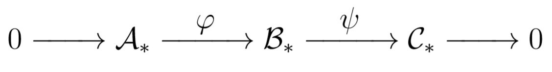
These maps give us the following diagram:
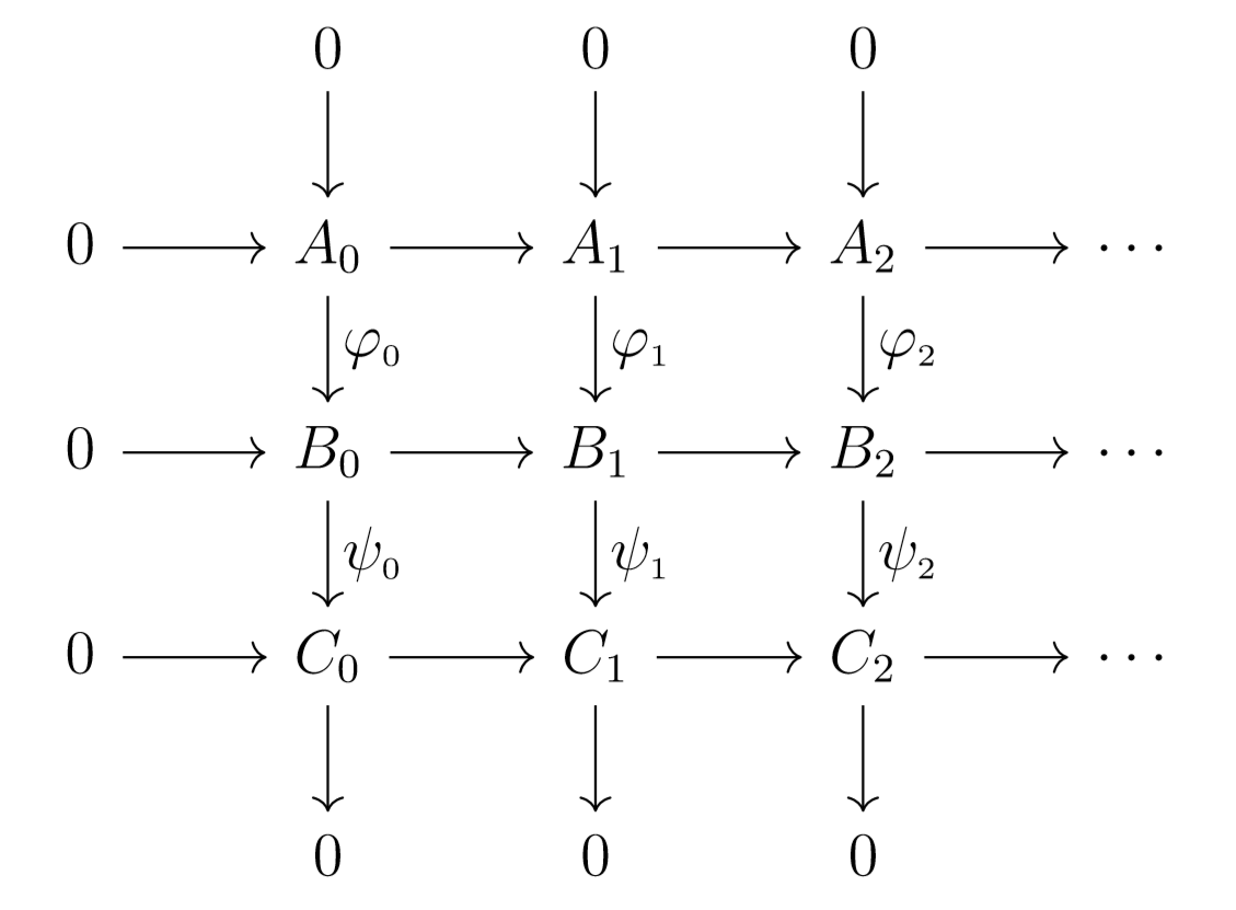
Note that if our first sequence is exact, then each sequence
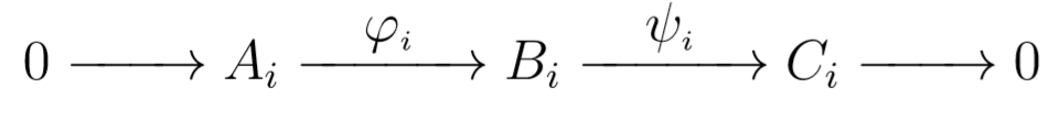
must be exact as well. This fact can sometimes assist us in computing homology groups.
Recall that each \(C_i\) is an abelian group, which provides the normality of all subgroups. This is crucial, because it allows us to finally reach the definition of a homology group that we’ve been building up for so long.
Definition: Let \(Z_n(\mathcal{K}) = \text{ker}(\partial_n)\) and \(B_n(\mathcal{K}) = \text{im}(\partial_{n+1})\). Define the \(n^\text{th}\) homology group of \(\mathcal{K}\) over \(G\) as \[H_n(\mathcal{K}; G) = Z_n(\mathcal{K})/B_n(\mathcal{K})\]
It is easy to see that \(H_n(\mathcal{K}, G)\) is in-fact an abelian group. In the common case that \(G = \mathbb{Z}\), we simply write \(H_n(\mathcal{K})\) for the \(n^\text{th}\) homology group of \(\mathcal{K}\). In the case that our chain complex forms an exact sequence, we have all homology groups \(H_n(\mathcal{K}; G) = 0\). This is known as trivial homology.
The idea of persistent homology as it applies to data analysis stems from the theory of simplicial homology we have just expounded. From a high-level perspective, the general idea is to construct simplicial complexes from data sets to attain topological objects for which we can compute homology and attain some understanding of a greater structure. While simplicial homology seems purely algebraic in nature, the ideas we will present for the persistent formulation of the theory have a nice geometric bend which makes interpreting our results relatively simple and intuitive. All of the algebraic objects we will be considering from this point on have clear geometric interpretations, and relatively easily pictured ones at that!
We will assume for the sake of simplicity that all points in our data sets will take values in \(\mathbb{R}\), so we get data that resides in \(\mathbb{R}^k\) where \(k\) is the number of relevant predictors. While there are likely an infinite number of ways to take a set of data and define a simplicial complex from it, perhaps the most natural and least computationally expensive way involves defining each point as a vertex, and making connections depending on some prescribed distance. We consider \(\mathbb{R}^k\) with the Euclidean topology for our purposes, which allows us access to the Euclidean metric for distance. Note however that in an abstract sense any metrizable topological space should work without issue, as we try to avoid any steps which specifically require \(\mathbb{R}^k\) with the Euclidean metric in particular.
More formally, we can define the particular simplicial complex of interest as such:
Definition: Let \(\mathbb{D} = \{ x_\alpha \}_\alpha\) be a set consisting of points in \(\mathbb{R}^k\), and choose a distance \(d \in \mathbb{R}\). The Vietoris-Rips complex, \(\mathcal{R}_d(\mathbb{D})\), is the simplicial complex with \(n\)-simplices corresponding to (\(n+1\))-tuples \(\{x_\alpha\}_{\alpha=0}^n\) falling within distance \(d\) of one and other pairwise. This is commonly (and more compactly) known simply as the Rips complex of \(\mathbb{D}\). For brevity, if the set \(\mathbb{D}\) is fixed and known we simply write \(\mathcal{R}_d\) to denote the relevant complex.
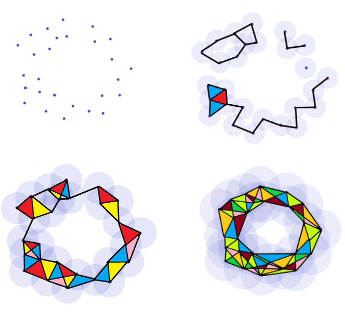
As a toy example, we will be considering the following set of points, \(\mathbb{D}\), sampled from an annulus:
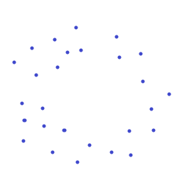
We choose a distance \(d\) which will be used to construct \(\mathcal{R}_d(\mathbb{D})\), and represent this distance by the purple disk about each point. We then connect each point whose disks overlap to arrive at the relevant Rips complex.
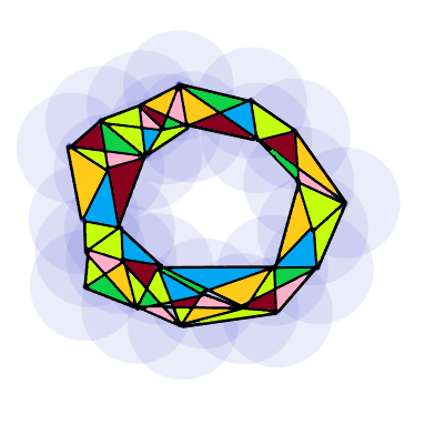
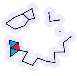
Note however that \(d\) was chosen carefully as to show the hole in the data through a nearly perfectly illustrative simplicial complex. The question immediately arises then as to how one chooses \(d\) to provide good results. If \(d\) is chosen to be too small, we get a complex comprised entirely of discrete points which is precisely \(\mathbb{D}\). On the other hand, if we choose a \(d\) that is too large it is easy to see that we get one giant simplex which will relay no information about potential holes in \(\mathbb{D}\) at all. As we vary our choice for \(d\), the complexes \(\mathcal{R}_d\) will reveal and hide various small holes on \(\mathbb{D}\) as points slowly branch out an connect to one and other. For example, suppose we chose a value for \(d\) only slightly smaller in diameter than that of the image above. Then we get an image with two smaller holes not seen in the above representation.
This brings us to the persistence in persistent homology. Generally speaking, our strategy is to vary \(d\) continuously and see which holes persist for notably long periods of time. These holes are likely to be relevant features of the data instead of transient quirks arising from poorly representative choices of \(d\). Suppose we choose increasing values of \(d\) indexed by \(i\), giving us a sequence \(\{d_i\}_{i=1}^n\). Since \(d_i < d_{i+1}\), it follows that \(\mathcal{R}_{d_i} \subseteq \mathcal{R}_{d_{i+1}}\). This gives us a chain of inclusions
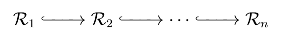
which looks quite similar to the chain complexes we have run into before.
Definition: Each hole arising in our chain complex first appears at some value, say \(d_\alpha\). Because a large enough choice for \(d\) will always provide us with a single simplex, there must be some distance \(d_\zeta\) for which this hole disappears. We can define the persistence of the hole then as the interval \([d_\alpha, d_\zeta]\). This allows us to quantify roughly how significant of a feature each hole is.
Each of these intervals is a bar in a larger geometric object known as a barcode. These barcodes allow us to see which holes are genuine features of a data set, and which exist due to conditions caused by variations in the distance parameter. We can actually characterize these barcodes purely algebraically by constructing a persistence module and computing its homology. To do this, we first create a persistence complex from our Rips complexes and endow it with some extra structure.
Definition: A persistence complex is a sequence of complexes \(\mathcal{C} = (C_*^i)_i\) with maps \(x \colon C_*^i \rightarrow C_*^{i+1}\). This is a generalization of the situation we currently have with Rips complexes, simply replace \(\mathcal{C} = (C_*^i)_i\) by \(\mathbf{R} = (\mathcal{R}_{d_i})_i\) and \(x\) by the inclusion. We will be performing the rest of the algebraic exposition using \(\mathcal{C}\) for the sake of generality.
These mappings, \(x\), induce homomorphisms on the homology groups of the persistence complexes. These homology groups make up the persistent homology of \(\mathbf{R}\).
Definition: The \((i,j)\)-persistent homology of \(\mathcal{C}\), \(H_*^{i \rightarrow j}(\mathcal{C})\), is given by image of \[x_* \colon H_*(C_*^i) \rightarrow H_*(C_*^j)\]
Of course, computing the homology of \(\mathcal{C}\) is no simple task. While wading through the necessary sea of homological algebra to accomplish this may be daunting for a mathematician, it is nearly impossible for a machine to do on first principles. Instead, we need to equip \(\mathcal{C}\) with additional structure to allow us to easily classify its homology. Let \(\mathbb{F}\) be some fixed field. As far as the algebra is concerned any field will work, but from a computational standpoint it is best to stick with something small such as \(\mathbb{Z}/2\mathbb{Z}\). We can equip \(\mathcal{C}\) with the structure of a graded \(\mathbb{F}[x]\)-module, where the action of \(x \in \mathbb{F}[x]\) works to shift the \(C_*^i\)’s. We then arrive at a classification for the homology of \(\mathcal{C}\) over \(\mathbb{F}\):
Theorem: Let \(\mathcal{C}\) be a persistence complex endowed with an \(\mathbb{F}[x]\)-module structure. Then the structure of the homology of \(\mathcal{C}\) is given by \[H_*(\mathcal{C}; \mathbb{F}) \cong \bigoplus_i x^{t_i} \cdot \mathbb{F}[x] \oplus \left( \bigoplus_j x^{r_j} \cdot \left( \mathbb{F}[x]/(x^{s_j} \cdot \mathbb{F}[x]) \right) \right)\]
Here, \(t_i\) corresponds to homology generators (i.e. holes) who appear at \(i\) and persist over \(i\). Moreover, \(r_j\) and \(s_j\) are parameters which signal generators appearing at \(r_j\) and disappearing at \(r_j + s_j\). This more rigorous algebraic treatment allows a (relatively) easy decomposition and classification of the homology of the module. Also note that \(\mathcal{C}\) can be decomposed into individual bars \[\mathcal{C} = \bigoplus_j \mathcal{C}^{I_j}\]
where each \(C^{I_j}\) is a module representing some bar in our bar code. In the next post, we will use a Python package, Dionysus, to perform some data analysis using persistent homology.