Demonstration of Persistent Homology
This is a follow up to the previous post detailing the basic mathematics behind persistent homology. A few basic applications will be demonstrated.
Now that we’ve dissected some of the basic algebraic facets of persistent homology in the previous post, we can apply these tools to some real data using a persistent homology package, Dionysus. In particular, the following data analysis was performed using the anaconda suite for Python 3. In our first example, we sample points from an annulus which we’ve randomly generate using the normalization of NumPy arrays. The annulus used looks like so:
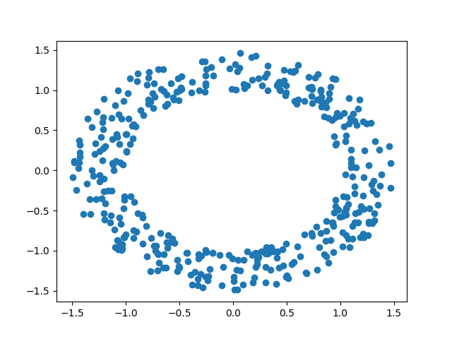
We then apply Dionysus to the annulus to generate a Rips filtration. The filtration obtained uses a max distance parameter of of 2, and has 2,997,920 simplices overall. The persistent homology of the annulus was computed using the following code:
import dionysus._dionysus as d
import dionysus.plot as plot
import numpy as np
# Get random points normally distributed
coords = np.random.normal(size = (400, 2))
# Generate annulus
for i in range(coords.shape[0]):
coords[i] = (coords[i] / np.linalg.norm(coords[i], 2)) * np.random.uniform(1, 1.5)
# Generate the Rips filtration
rips_filtration = d.fill_rips(coords, 2, 2)
# Compute the persistent homology of the filtration
persistence = d.homology_persistence(rips_filtration)
# Initialize diagrams
diag = d.init_diagrams(persistence, rips_filtration)
# Show bar diagram
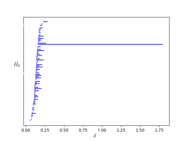
plot.plot_bars(diag[1], show = True)
The output of this code was a bar diagram which very clearly showed a central hole with a very high rate of persistence. As such, we can ascertain from this data that the central hole is in-fact a relevant feature, and not just a function of noise.
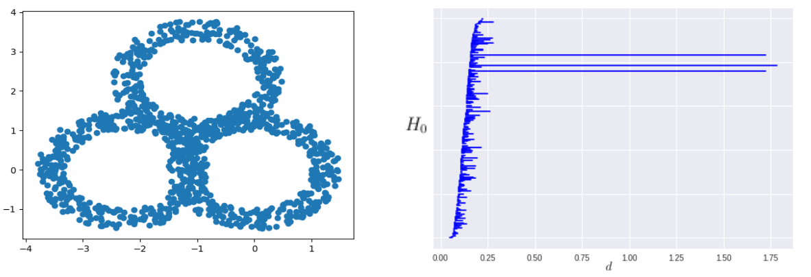
Using a similar process we generated three copies of the initial annulus, positioning them as to form a single triple-annulus strucutre. We can also perform the above calculation in precisely the same way for a 1200 point triple annulus over a filtration of 66,453,220 simplices. This produced a barcode which very clearly shows the three obvious holes, highlighting them as relevant features of the data.
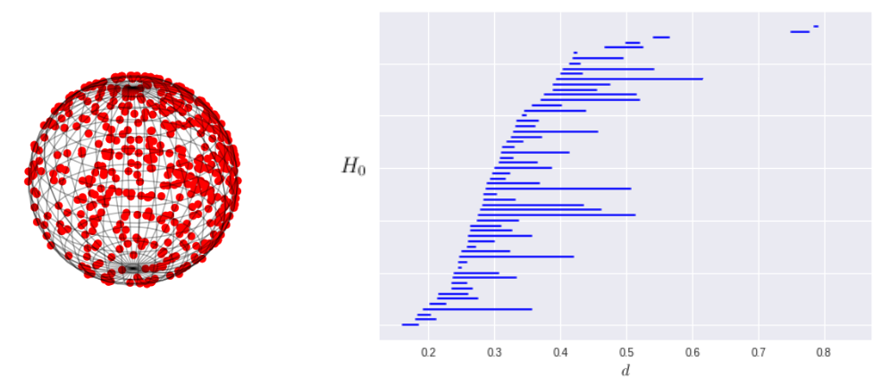
We can also compute the persistent homology of figures in higher dimensions than 2. We generated a sphere using the VonMisesFisher distribution that can be found in the Tensorflow probability package.
import dionysus._dionysus as d
import dionysus.plot as plot
import tensorflow as tf
import tensorflow_probability as tfp

# Setup tensorflow environment and import distributions
tf.enable_eager_execution()
tfd = tfp.distributions

# Randomly select points on a unit sphere using the VMF distribution
vmf = tfd.VonMisesFisher(mean_direction=[0., 1, 0], concentration=1.)
sphere = vmf.sample(200).numpy()

# Compute filtration
rips_filtration = d.fill_rips(sphere, 3, 2)

# Compute persistence and initialize diagram
persistence = d.homology_persistence(rips_filtration)
diag = d.init_diagrams(persistence, rips_filtration)

# Show the bar diagram
plot.plot_bars(diag[1], show = True)
This calculation required a filtration of 60,245,421 simplices and produced a persistence diagram matching what we would expect for the homology of a sphere. Note that the code is very similar to what is found in the calculation for each of the annular data sets, but the Rips complex is generated in 3 dimensions instead of two.
The computations performed above utilized data sets which were relatively dense, and whose shape was very distinct. Persistent homology works best under these conditions, but does not require such clean data sets. To verify this, we can reduce the point density of our single and triple annulus examples. This gives us something which is still geometrically intuitive, but the main hole is not so clear in more minimal cases. We considered the singular annulus over 100, 50, and 25 points, all of which gave good results.
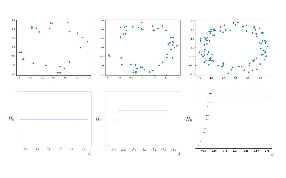
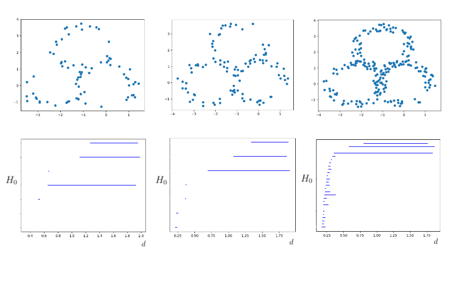
We had similarly good results when considering the triple annulus over 225, 105, and 75 points. In some instances these smaller data sets actually had clearer homology due to the reduction in noise picked up by the filtration. The sparsity of the points reduced the likelihood of finding holes which were non-relevant. Reducing the size of the data set also had the benefit of drastically speeding up the computation. These reduced sets all had filtrations with less than 25,000 simplices, some of which had filtrations with as little as 7000. This was able to reduce the computation time from upwards of 20 minutes to as little as 2 seconds.
In the next post, we will discuss the theory of algebraic varieties as it applies to data analysis and algebraic statistics.