A Basic Statistical Primer
The following is a basic statistical primer which can be used to help guide the reading of the rest of this blog. It touches upon basic statistical concepts such as bias, variance, probability spaces, random variables, etc.
In many of the derivations and discussions on this blog we will use notation and terminology common to probability theory and statistical learning theory. As such, I think it is fitting that I provide a basic statistical primer outlining that information. The discussion here will vary in brevity, as explanations will be given in further detail on separate posts when practical.
First, we’d like to develop the notion of a probability space; a collection consisting of a sample space, probability measure, and \(\sigma\)-algebra.
Definition: A sample space, \(\Omega\), is the set of all possible outcomes arising from an experiment.
In general, we will consider all sample spaces discussed to be finite or countably infinite. We will deal with cases of uncountably infinite sample spaces separately as they arise (this is a far more interesting topic, but not necessarily one which should be addressed in a basic primer).
Definition:A \(\sigma\)-algebra over a sample space \(\Omega\) is a subset \(\mathcal{F} \subset \mathcal{P}(\Omega)\) satisfying the following criteria:
- The relationship \(\Omega \in \mathcal{F}\) holds
- If \(U \in \mathcal{F}\), then \(U^\text{c} \in \mathcal{F}\)
- If a countable number of subsets \(U_1, U_2, \ldots \in \mathcal{F}\), then their union \(\bigcup_{i=1}^\infty U_i \in \mathcal{F}\)
This definition can be somewhat abstract, so we can clarify things with an example. For intuition, we will consider a finite sample space \(\Omega\) and equip it with a \(\sigma\)-algebra, \(\mathcal{F}\). Let \(\Omega = \{1, 2, 3, 4\}\), and \(\mathcal{F} = \{ \emptyset, \{1, 2\}, \{3, 4\}, \{1, 2, 3, 4\} \}\). Clearly \(\Omega \in \mathcal{F}\), each \(U \in \mathcal{F}\) has a corresponding complement, and \(\mathcal{F} \subset \mathcal{P}(\Omega)\). Notice then that the choice of \(\sigma\)-algebra for a given sample space is not unique. The power set itself, \(\mathcal{P}(\Omega)\), is actually an example of a \(\sigma\)-algebra on \(\Omega\). Of course, \(\Omega \in \mathcal{P}(\Omega)\) as well as all necessary complements, so no proof is necessary. We can also compare this to the simplest possible \(\sigma\)-algebra, \(\mathcal{F}_{\text{discrete}} = \{ \emptyset, \Omega \}\). This choice of \(\mathcal{F}\) is almost never used, but can sometimes be worth considering in pathological cases.
While the above example demonstrates that the choice of \(\sigma\)-algebra is not necessarily unique, there are natural constructions to consider that are often used in statistical theory. We can always assign \(\mathcal{P}(\Omega)\) and \(\mathcal{F}_{\text{discrete}}\) to a sample space, but these choices are not always useful or manageable. More frequently, we are interested in the \(\sigma\)-algebra induced by some topology. The notion of a topological space is related to the pair \((\Omega, \mathcal{F})\) by the construction of a Borel algebra.
If we consider a collection \(\{ \mathcal{F}_i \mid i \in I \}\) where \(I\) is an indexing set and each \(\mathcal{F}_i\) is a \(\sigma\)-algebra over \(\Omega\), we can obtain a new \(\sigma\)-algebra by intersecting the \(\mathcal{F}_i\) over \(I\) like so \[\mathcal{F}^* = \bigcap_{i \in I}\mathcal{F}_i\]
To see that \(\mathcal{F}^*\) is truly a \(\sigma\)-algebra is not too difficult. We can generalize this idea to arbitrary subsets of \(\mathcal{P}(\Omega)\). In particular, given a subset \(\Gamma \subset \mathcal{P}(\Omega)\), we have a \(\sigma\)-algebra \[\mathcal{F}(\Gamma) = \bigcap \{ \mathcal{F} \mid \Gamma \subseteq \mathcal{F} \}\]
Here, \(\mathcal{F}(\Gamma)\) is the interesection of all \(\sigma\)-algebras over \(\Omega\) containing \(\Gamma\). This construction is useful because it is naturally the smallest \(\sigma\)-algebra containing \(\Gamma\). We can use our above construction to link topological spaces to probability spaces. Suppose we have \((\Omega, \tau)\) where \(\tau\) is some topology on \(\Omega\). Because \(\tau\) is simply a collection of sets, we define \(\mathscr{B}_\Omega \coloneqq \mathcal{F}(\tau)\) to be our Borel \(\sigma\)-algebra. This is a much more natural construction which respects the overarching topology of the space, and has the property of being the smallest \(\sigma\)-algebra with respect to that topology. One case to keep in mind for choosing \(\sigma\)-algebras is that of finite \(\Omega\). In particular, \(\mathcal{P}(\Omega)\) is the Borel algebra for finite \(\Omega\), and as such is used widely under those circumstances.
Definition: Let \(\Omega\) be a sample space, and \(\mathcal{F}\) a \(\sigma\)-algebra on \(\Omega\). A probability measure on the pair \((\Omega, \mathcal{F})\) is a mapping \[\begin{aligned} P \colon & \mathcal{F} \longrightarrow [0, 1] \\ & U \longmapsto P(U) \end{aligned}\]
with with \(P(\Omega) = 1\) and \[P \left( \bigcup_{i=1}^\infty U_i \right) = \sum_{i=1}^\infty P(U_i) \ \ \text{if} \ \ U_i \cap U_j = \emptyset \ \ \forall i \neq j\]
In the theory of statistical modeling, the notion of conditional probability is extremely important. Now that we have an understanding of probability spaces, we define conditional probabilities and move on to random variables.
Definition: Let \((\Omega, \mathcal{F}, P)\) be a probability space with \(A, B \in \mathcal{F}\) and \(P(B) > 0\). We say the conditional probability of \(A\) given \(B\) is \[P(A \mid B) = \frac{P(A \cap B)}{P(B)}\]
Definition: A random variable on a probability space \((\Omega, \mathcal{F}, P)\) is a function \(X \colon \Omega \rightarrow \mathbb{R}\) with the property that for all measurable sets \(B\), \(X^{-1}(B) \in \mathcal{F}\). We say \(X\) is discrete if \(\Omega\) is finite, and continuous otherwise.
We now have the most basic building blocks of statistics constructed. From this we can begin to understand bias and variance. Error in model construction and prediction (aside from the irreducible error) takes two main forms; bias and variance. Shortly we will see precisely how these components fit into the mathematical definition of error, but first we give a more intuitive understanding. Given a response, \(y\), we can assume there is some true model \(f(\bm{X}) + \varepsilon\) which takes values in a set of observations and predicts \(y\). Through various algebraic and statistical methods we can determine a model, \(\hat{f}\), for \(f\). The bias of \(\hat{f}\) is the discrepancy between the values of \(\hat{f}(\bm{X})\) and \(f(\bm{X})\). This bias component of error refers to how far a model is from correctly predicting the response variable, \(y\). Formally, bias is the discrepancy between the expected value of a model and true value being estimated.
Definition: A density function is an integrable function \(\psi \colon \mathbb{R}^n \rightarrow [0, \infty)\) such that \[\int_{\mathbb{R}^n}\psi (x)dx = 1\]
Given a random variable, \(X\) and a density, \(\psi\), we often want to know the expected value of \(X\). This expected value captures the average predicted value of the random variable. More precisely:
Definition: Let \((\Omega, \mathcal{F}, P)\) be a probability space and \(X\) a random variable in \(\Omega\) with finite range. If \(\Omega\) is finite we define the expected value of \(X\) as \[E[X] = \sum_{x \in \mathbb{R}} xP(X = x)\]
In the case of \(X\) having infinite range, we have \[E[X] = \int_\Omega XdP\]
which, if \(\Omega \subseteq \mathbb{R}\), is equivalent to \[E[X] = \int_\mathbb{R} x \psi (x)dx\]
Note that in the above \(\psi\) is the density of \(X\). We can use this notion of expected value to more precisely understand bias and variance.
Definition: Let \(\hat{f}\) be a model for \(f\). The bias of \(\hat{f}\) is given by \[\text{Bias}(\hat{f}) = E[\hat{f} - f] = E[\hat{f}] - E[f]\]
Note that we are treating \(\hat{f}\) and \(f\) as random variables in this context.
Variance on the other hand is a measure of how widely-ranging predictions are given a particular point. It is explained mathematically as the expected value of the squared deviation from the mean of a random variable. We can define variance formally in the following way:
Definition: For a random variable, \(X\), the variance of \(X\) is given by \[\text{Var}(X) = E\left[\left(X - E[X]\right)^2\right] = E[X^2] - E[X]^2\]
It is possible to have highly biased models with low variance, highly variant models with low bias, or something in between. Particularly, the relationship between bias and variance is driven by model complexity, specifically as models get more complex the bias tends to decrease, while the variance tends to increase. In more intuitive terms, highly variant models are excellent at capturing the properties of a training set but when used to predict new data they tend to run into trouble with overfitting, i.e. sticking too closely to the training set. Highly biased models on the other hand tend to be very simple and usually run into trouble with underfitting, which is the failure to properly capture important features of the data set.
Bias and variance are not solely features of the chosen model, and can be controlled not only by changing the structure of the model, but also the structure of the observed data. For example, if we choose to increase the size of the training set used to construct \(\hat{f}\), we would see a decrease in variance. We will see examples of what overfitting and underfitting look like, but first we decompose total error into bias and variance components.
We can turn to a simple model \(y = f(X) + \varepsilon\) with predicted function \(\hat{f}\). If we let \(\text{Var}(\varepsilon) = \sigma_\varepsilon^2\) then we can perform an error decomposition at \(X = x\) for \(\hat{f}\) in the following way: \[\begin{aligned} \text{Err}(x) &= E\left[\left(y - \hat{f}(x)\right)^2 \ \biggm\vert \ X = x\right] \\ &= \left(E\left[\hat{f}(x)\right] - f(x)\right)^2 + E\left[\hat{f}(x) - E[\hat{f}(x)]\right]^2 + \sigma_\varepsilon^2 \\ &= \text{Bias}^2\left(\hat{f}(x)\right) + \text{Var}\left(\hat{f}(x)\right) + \sigma_\varepsilon^2 \end{aligned}\]
This allows us to decompose our total error into squared-bias, variance, and irreducible error. The ultimate goal is to minimize bias and variance related error, but unfortunately in the real world it is nearly impossible to achieve 0 bias and variance error. Now that we have a more targeted mathematical description of bias and variance, we can consider some simple graphical examples.
Example: In this example, we generate values from a cubic function using R, making sure to add noise to reduce the obviousness of the shape.
x <- runif(30,  min=-9, max=9)
y <- 10 - x - 0.6 * x^2 + 0.4 * x^3 + rnorm(length(x), 0, 8)
plot(x, y, [plotArgs])
Here we see that the data points are generated using the target function \(.4x^3 - .6x^2 - x - 10\) with added noise. We then generate a model of the form \(\hat{f}_k = \sum_{i=0}^k \beta_i x^i\) where \(k\) is the desired degree. In our case, \(\text{deg}(f) = 3\), so the right level of complexity for \(\hat{f}\) would involve using a degree 3 function. To illustrate the relationship between bias, variance, and function complexity we can consider models of varying degrees.
We have the following code used to generate the bias and mean squared error values:
meanSquaredError = function(f_est, f_x){
	mean((f_est - f_x)^2)
}

biasError = function(f_est, f_x){
	mean(f_est) - f_x
}
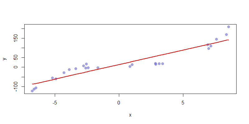
These functions take output from \(\hat{f}\) and \(f\) to generate the mean squared error and bias. We can already calculate variance using a built-in R function. First, we have \(\hat{f}_1\) consisting of a monomial \(\alpha + \beta x\). We can see that this function is not complex enough to accurately capture the features of the data set. As a result, \(\hat{f}_1\) is highly biased and has almost no variance.
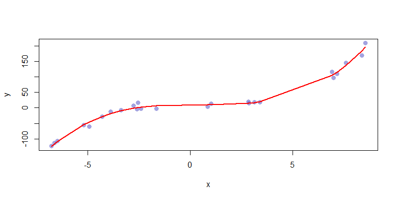
If we consider the most natural choice, \(\hat{f}_3 = \sum_{i=0}^3 \beta_i x^i\) we get a model which has an acceptable mix of bias and variance. The complexity here is a good fit for the presented data, and captures all of the relevant features of the data set. This is an ideal fit.
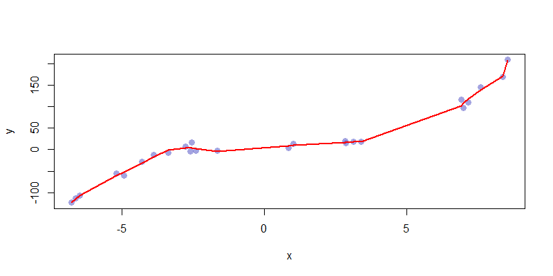
We can compare this nice fit to something which is highly variant, say \(\hat{f}_{12} = \sum_{i=0}^{12} \beta_i x^i\). This too closely captures the feature of the data set, making its predictive capabilities nearly useless. This is an example of a highly overfitted model.
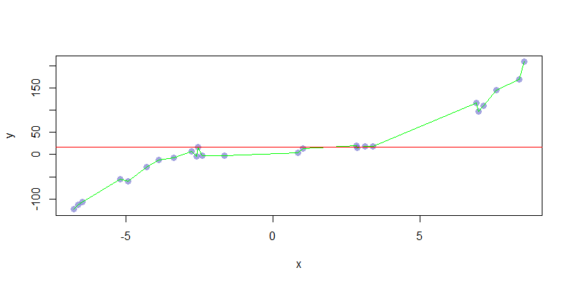
For the above models, notice that the bias decreased with model complexity, while variance did the opposite. It was at \(\hat{f}_3\) that we saw the best error rate, but not minimal levels of both bias and variance. Generally, we are unable to completely minimize both bias and variance at the same time. These are practical examples, but we can compare them to limit cases. The following chart shows \(\hat{f}_0 = \alpha\) and \(\hat{f}_\ell = \sum_{i=0}^\ell \beta_i x^i\) where \(\ell = \#\text{Observations} - 1\). These are models with maximal bias and variance, which leads to maximal under and overfitting.
We can perform some general calculations of the bias and variance involved in these maximal models. In particular: \[\begin{aligned} \text{Err}_{(\hat{f}_0)}(x) &= \text{Bias}^2\left(\hat{f}_0(x)\right) + \text{Var}\left(\hat{f}_0(x)\right) + \sigma_\varepsilon^2 \approx \text{Bias}^2\left(\hat{f}_0(x)\right) + \sigma_\varepsilon^2 \\ \text{Err}_{(\hat{f}_\ell)}(x) &= \text{Bias}^2\left(\hat{f}_\ell(x)\right) + \text{Var}\left(\hat{f}_\ell(x)\right) + \sigma_\varepsilon^2 \approx \text{Var}\left(\hat{f}_\ell(x)\right) + \sigma_\varepsilon^2 \end{aligned}\]
Note that regardless of the \(\hat{f}\) used, there will always be error. In fact, if we tried to make predictions using the true function \(f = .4x^3 - .6x^2 - x - 10\), we would still see error due to noise in the data. As such, the goal is simply to dually minimize both squared-bias and variance error to achieve the closest possible fit.